标签：varnish series range client Down Prometheus PromQL time

 

原文：https://www.section.io/blog/prometheus-querying/

 

https://www.cnblogs.com/wayne-liu/p/9273452.html   这篇文章里面讲的还有些没弄懂？？到底有些运算有什么用，什么应用场景？

---------------------------------------------------------------------

 

Prometheus has its own language specifically dedicated to queries called PromQL. It is a powerful functional expression language, which lets you filter with Prometheus’ multi-dimensional time-series labels. The result of each expression can be shown either as a graph, viewed as tabular data within Prometheus’ own expression browser, or consumed via external systems via the HTTP API.

PromQL can be a difficult language to understand, particularly if you are faced with an empty input field and are having to come up with the formation of queries on your own. This article is a primer dedicated to the basics of how to run Prometheus queries.

You will need only three tools:

• Prometheus server port forwarded from the local connection
• Simple cURL
• A data visualization and monitoring tool, either within Prometheus or an external one, such as Grafana

Through query building, you will end up with a graph per CPU by the deployment.

Prometheus Querying

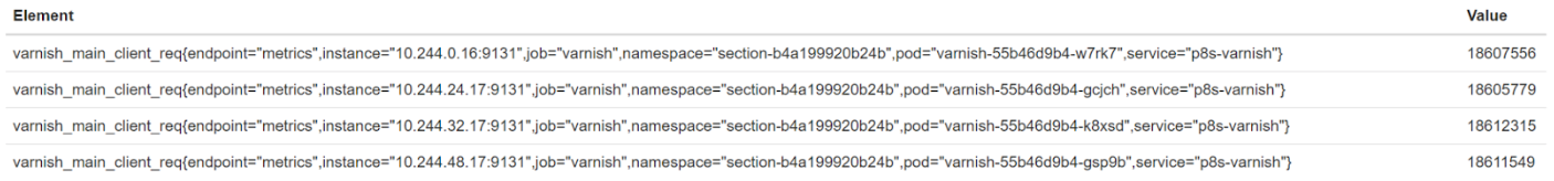
The core part of any query in PromQL are the metric names of a time-series. Indeed, all Prometheus metrics are time based data. There are four parts to every metric. Taking the varnish_main_client_req metric as an example:

The parts are:

1. Metric_name (e.g. varnish_main_client_req)
2. One or more labels, which are simply key-value pairs that distinguish each metric with the same name (e.g. namespace="section-b4a199920b24b"). Each metric will have at least a job label, which corresponds to the scrape config in the prometheus config.
3. The value, which is a float64. When querying in the Prometheus console, the value shown is the value for the most recent timestamp collected.
4. The timestamp, which has millisecond precision. The timestamp doesn’t appear in the query console, but if you switch to the Graph tab within Prometheus, you can see the values for each timestamp in the chart.

Each distinct metric_name & label combination is called a time-series (often just called a series in the documentation). If each series only has a single value for each timestamp, as in the above example, the collection of series returned from a query is called an instant-vector. If each series has multiple values, it is referred to as a range-vector. These are generated by appending a time selector to the instant-vector in square brackets (e.g. [5m] for five minutes). The instant vector and range vector are two of four types of expression language; the final two are scalar, a simple numeric floating point value, and string, a simple string value. See Range Selectors below for further information on this.

All of these metrics are scraped from exporters. Prometheus scrapes these metrics at regular intervals. The setting for when the intervals should occur is specified by the scrape_interval in the prometheus.yaml config. Most scrape intervals are 30s. This means that every 30s, there will be a new data point with a new timestamp. The value may or may not have changed, but at every scrape_interval, there will be a new datapoint.

There are four types of metrics:

• Counters - A cumulative, monotonic metric. Counters allow the value to either go up, stay the same or be reset to 0 (on a process restart). varnish_main_client_req is an example of this, which provides the total number of HTTP requests that the varnish instance has handled in its life.
• Gauges - A non-monotonic metric. Gauges can go either up or down, giving the current value at any given point in time. An example is node_memory_utilisation, which provides the current percentage of memory used on each node.
• Histogram - This creates multiple series for each metric name. Sampled values are put into buckets. Sum & count metrics are also generated for each sample.
• Summary - The summary is similar to histogram in that it takes samples and creates multiple metrics, including sum & count. However, it creates quantiles (i.e. 50th percentile, 90th percentile, etc.) instead of buckets.

We’re going to deal with counters for this analysis, as it’s the most common metric type.

Query Structure

The structure of a basic Prometheus query looks very much like a metric. You start with a metric name. If you just query varnish_main_client_req, every one of those metrics for every varnish pod in every namespace will get returned. If you do this in Grafana, you risk crashing the browser tab as it tries to render so many data points simultaneously.

Next, you can filter the query using labels. Label filters support four operators:

• = equal
• != not-equal
• =~ matches regex
• !~ doesn’t match regex

Label filters go inside the {} after the metric name, so an equality match looks like:

varnish_main_client_req{namespace="section-9469f9cc28d8d"}

which will return only varnish_main_client_req metrics with that exact namespace.

Regex matches use the RE2 syntax. If you’re familiar with PCRE, it will look much the same, but it doesn’t support backreferences (which really shouldn’t matter here anyway).

You can also use multiple label filters, separated by a comma. Multiple label filters are an “AND” query, so in order to be returned, a metric must match all the label filters.

For instance, varnish_main_client_req{namespace=~".*3.*",namespace!~".*env4.*"} will return all varnish_main_client_req metrics with a 3 in their namespace that don’t also contain env4.

Range Selectors

By appending a range duration to a query, we get multiple values for each timestamp. This is referred to as a range-vector. The values for each timestamp will be the values recorded in the time series back in time, taken from the timestamp for the length of time given in the range duration.

As an example, take varnish_main_client_req{namespace="section-9469f9cc28d8d"}. If we add a [1m] range selector we now get this:

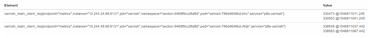
We get two values for each series because the varnish scrape config specifies that it has a 30 second interval, so if you look at the timestamps after the @ symbol in the value, you can see that they are exactly 30 seconds apart. If you graphed these series without the range selector and inspected the value of the lines at those timestamps, it would show these values.

Now, range-vectors can’t be graphed because they have multiple values for each timestamp. If you select the Graph tab in the Prometheus web UI on a range-vector, you’ll see this message:

Error executing query: invalid expression type "range vector" for range query, must be Scalar or instant Vector

A range-vector is typically generated in order to then apply a function to it to get an instant-vector, which can be graphed (only instant vectors can be graphed). Prometheus has many functions for both instant and range vectors. The more commonly used functions for working with range-vectors are:

• rate() - calculates the per-second average rate of increase of the time series in the range vector over the whole range.
• irate() - calculates the per-second average rate of increase of the time series in the range vector using only the last two data points in the range.
• increase() - calculates the increase in the time series per the time range selected. It’s basically rate multiplied by the number of seconds in the time range selector.

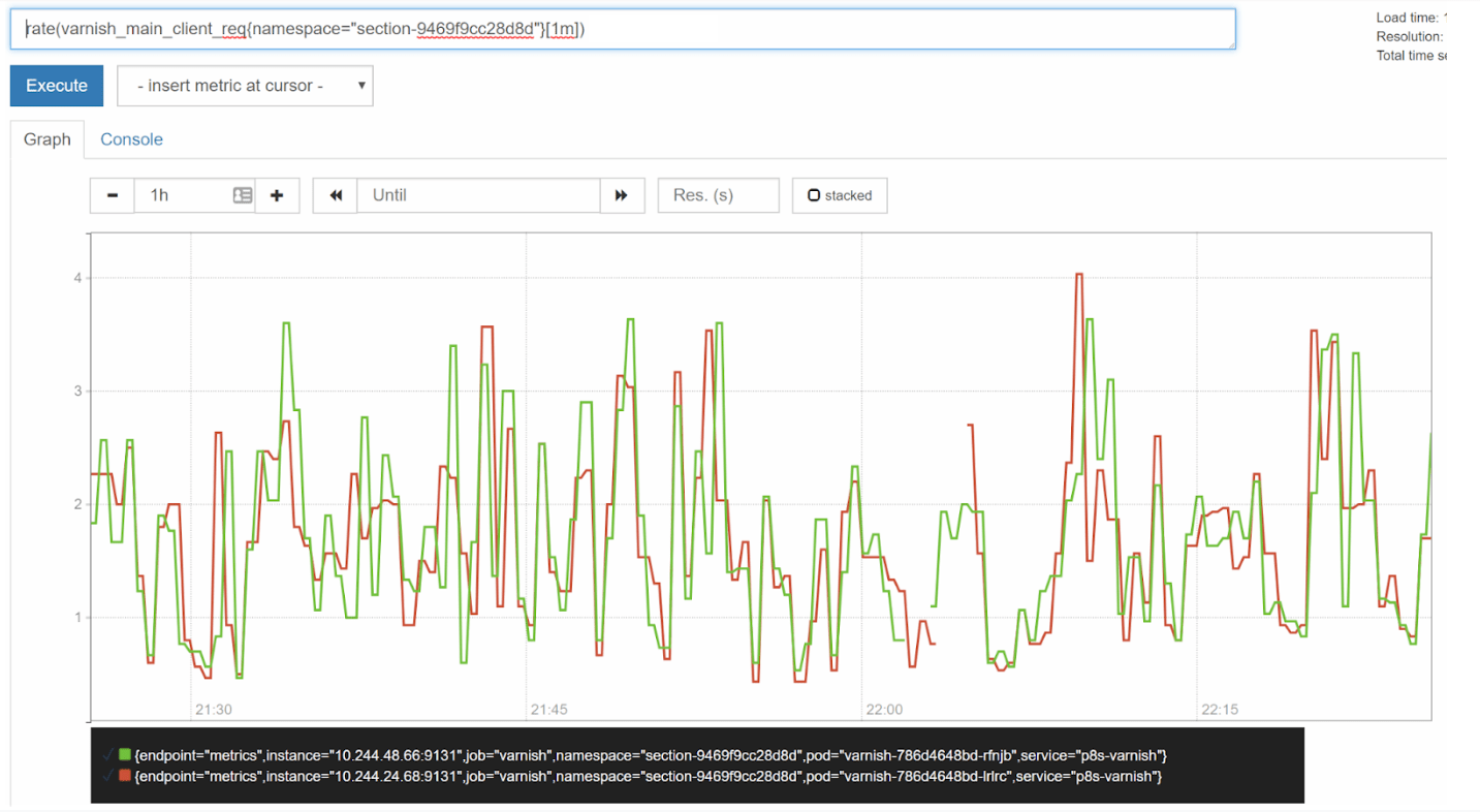
Your selection of range duration will determine how granular your chart is. A [1m] duration, for instance, will give a very spiky chart, making it difficult to visualize a trend, looking something like this:

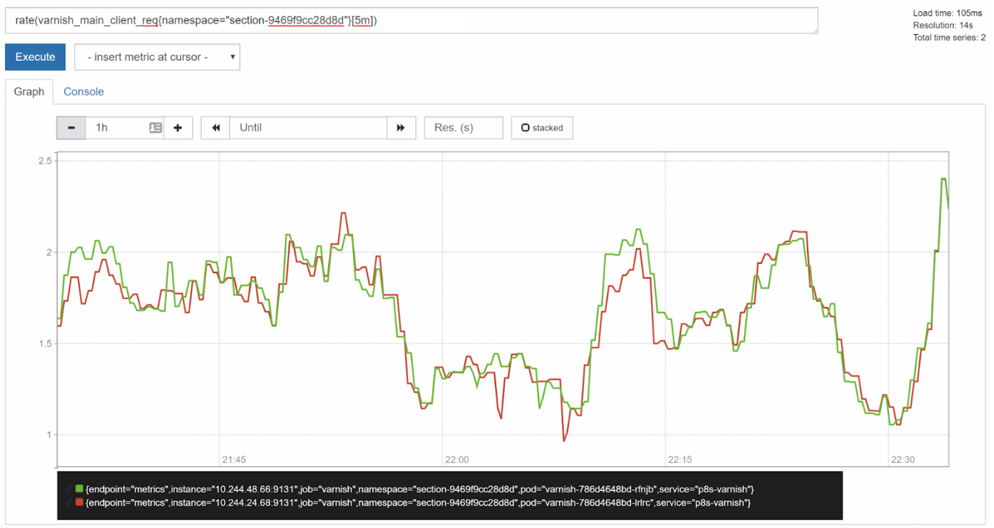
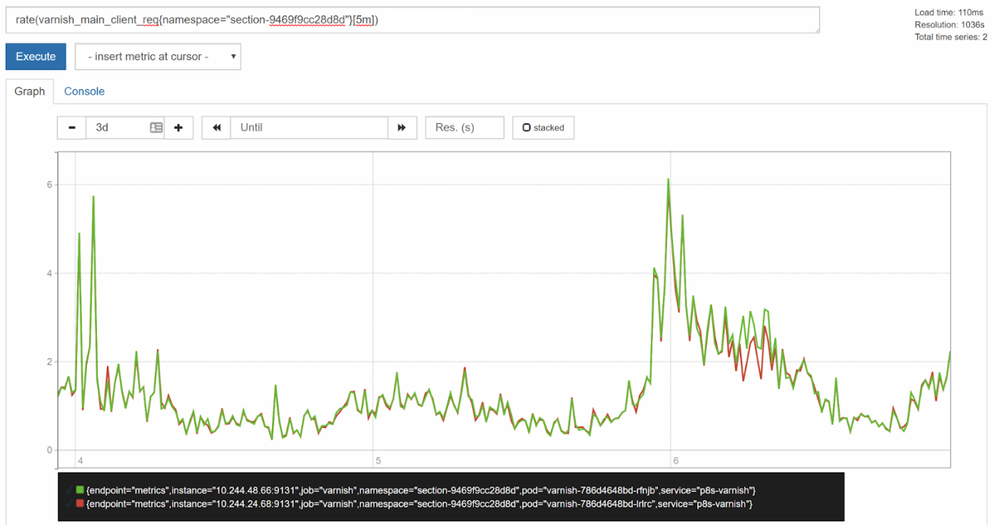
For a one hour view, [5m] would show a decent view:

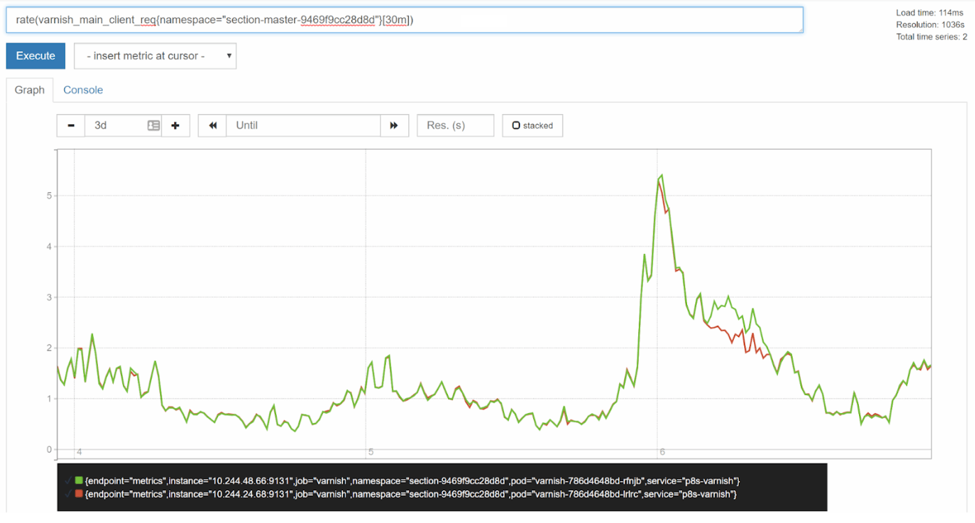
For longer time-spans, you may want to set a longer range duration to help smooth out spikes and achieve more of a long-term trend view. Compare the three day view with a [5m] duration to a [30m] duration:

Joining Series

Technically, Prometheus doesn’t have the concept of joining series like SQL, for example, has. However, series can be combined in Prometheus by using an operator on them. It has the usual arithmetic, comparison and logical operators that can be applied to multiple series or to scalar values.

A caution: if an operator is applied to two instant-vectors, it will only apply to matching series. A series is considered to match if and only if it has exactly the same set of labels. Using these operators on series achieves a one-to-one matching when each series from the left side of the expression exactly matches one series on the right side.

So, taking the two series from the previous examples as separate instant-vectors:

varnish_main_client_req{endpoint="metrics",instance="10.244.24.68:9131",job="varnish",namespace="section-9469f9cc28d8d",pod="varnish-786d4648bd-lrlrc",service="p8s-varnish"}

&

varnish_main_client_req{endpoint="metrics",instance="10.244.48.66:9131",job="varnish",namespace="section-9469f9cc28d8d",pod="varnish-786d4648bd-rfnjb",service="p8s-varnish"}

If we apply an addition operator to these two to try and get a total number of requests in that namespace, nothing will be returned.

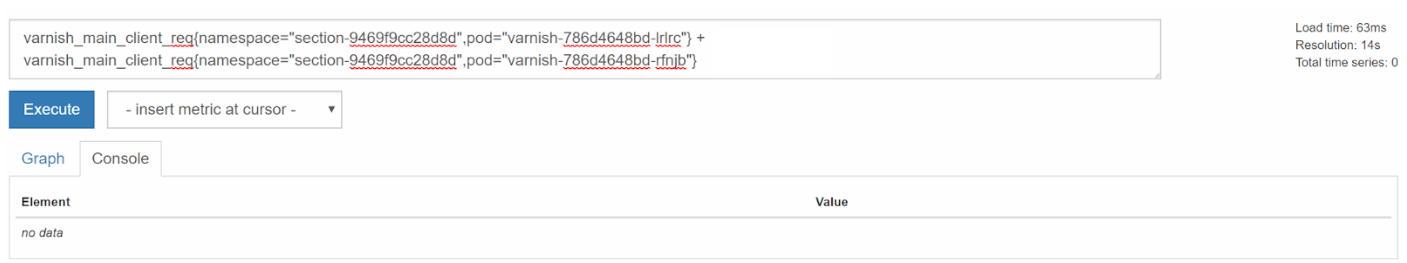
This is because there are no series returned that have exactly matching labels. However, if we use the on keyword to specify that we only want to match on the namespace label, we get:

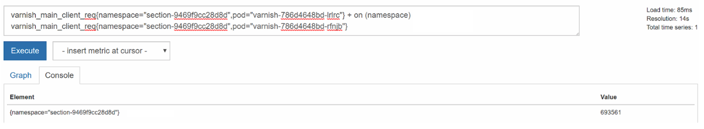
Note that the new instant-vector contains a single series with only the label(s) specified in the on keyword.

The ignoring keyword can also be used as an inverse of that to specify which labels should be ignored when trying to match.

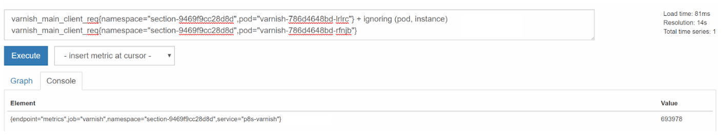
In this case the returned instant-vector contains a single series with all matching labels left after removing the labels in the ignoring set.

It is worth pointing out here that Prometheus also has a number of aggregation operators. So if we really wanted to get the total number of client requests in a namespace, we would never actually do this because the pod names would change over time. The sum operator is much simpler:

sum(varnish_main_client_req{namespace="section-9469f9cc28d8d"}) by (namespace)

Combining Instant-Vectors with Scalars

You can also combine an instant-vector with a scalar value. Each series in the instant-vector has the value applied with the operator. For example:

varnish_main_client_req{namespace="section-9469f9cc28d8d"} * 10

results in each value for each series in the instant-vector being multiplied by ten.

This can be useful for calculating ratios & percentages.

Kubernetes Reference Series

What if we wanted to know how many requests were being made against each node in our Kubernetes cluster? We can see this in the varnish_main_client_req series by looking at the instance label (e.g. instance="10.244.48.66:9131"). However, this is not particularly helpful as the IP address given there is only the internal IP address of the pod as addressed by the service the Prometheus operator has used to identify which endpoints to scrape. The port is t that which the varnishstat promethues exporter publishes its metrics endpoint to by default.

To address this, the kube-state-metrics and node-exporter Prometheus exporters publish a number of series that essentially exist to provide reference labels. These are series like kube_pod_info & node_uname_info.

There is a kube_pod_info series for every single pod in the cluster. If we filter it down to the two pods we are interested in knowing more about, we can see what kind of information it provides:

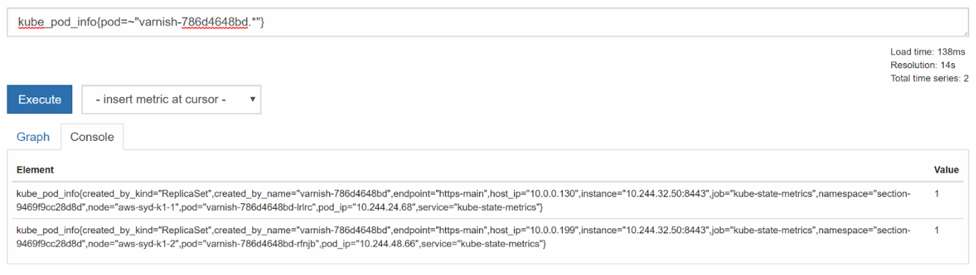
From this, we can see the name of the node, the IP address of the nodes and which ReplicaSet created the pods.

Also note the value. The value for these reference series is always 1. The reason for this is so that you can join them with other series simply by multiplying without having to change the value of the original series, and still gain access to the new set of labels.

So, to get our varnish_main_client_req series with the node label on them, we can do this :

varnish_main_client_req{namespace="section-9469f9cc28d8d"} * on (pod) kube_pod_info

This returns us:

Unfortunately because we needed to use the on keyword to match, that is also the only label we get back. Ignoring non matching labels won’t help here because pod is the only matching label. To fix this, we use the group_left or group_right keywords.

These keywords convert the match into a many-to-one or one-to-many matching respectively. The left and right indicate the side that has the higher cardinality. So a group_left means that multiple series on the left side can match a single series on the right. The result of this is that the returned instant-vector contains all of the labels from the side with the higher cardinality, even if they don’t match any label on the right.

So varnish_main_client_req{namespace="section-9469f9cc28d8d"} * on (pod) group_left() kube_pod_info gives:

This gives us back all the labels for the varnish_main_client_req series, however we still don’t have the node label. To solve this, the group_left and group_right keywords allow a label list to be passed in. The labels provided will be included from the matching lower cardinality side of the operation. So by doing:

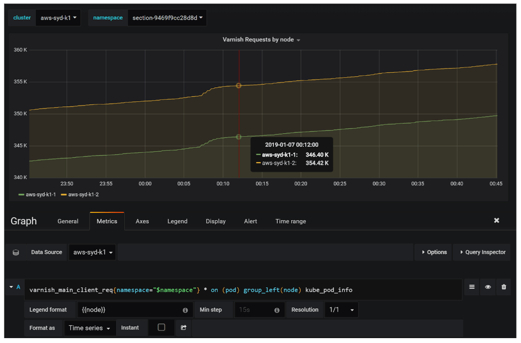
varnish_main_client_req{namespace="section-9469f9cc28d8d"} * on (pod) group_left(node) kube_pod_info

We can get all the information required:

We can then take this over to Grafana to make a dashboard and chart, add this data to a graph panel, and clearly view it all.

Avoiding Overloads and Slow Queries

Sometimes graphing a query might overload the server or browser, or lead to a time out because the amount of data is too large. When constructing queries over unknown data, it is better to begin building the query in the tabular view of Prometheus’ expression browser until you arrive at a reasonable result set (i.e. hundreds as opposed to thousands of time series). Switch to graph mode only once you have sufficiently aggregated or filtered your data. If the expression continues to take too long to graph ad-hoc, you can pre-cord it using a recording rule. This is particularly relevant to PromQL when a bare metric name selector such as api_http_requests_total can easily expand to thousands of time series each with a different label. Also, expressions that aggregate over multiple time series will generate load on the server even when the output is only a small amount of time series.

标签：varnish,series,range,client,Down,Prometheus,PromQL,time
来源： https://www.cnblogs.com/oxspirt/p/15015806.html

本站声明： 1. iCode9 技术分享网（下文简称本站）提供的所有内容，仅供技术学习、探讨和分享；
2. 关于本站的所有留言、评论、转载及引用，纯属内容发起人的个人观点，与本站观点和立场无关；
3. 关于本站的所有言论和文字，纯属内容发起人的个人观点，与本站观点和立场无关；
4. 本站文章均是网友提供，不完全保证技术分享内容的完整性、准确性、时效性、风险性和版权归属；如您发现该文章侵犯了您的权益，可联系我们第一时间进行删除；
5. 本站为非盈利性的个人网站，所有内容不会用来进行牟利，也不会利用任何形式的广告来间接获益，纯粹是为了广大技术爱好者提供技术内容和技术思想的分享性交流网站。